Continuous Variable Quantum Key Distribution

History and intuition

Around 2000, there were several proposals of using continuous variable for quantum key distribution. We will not discuss in great depth continuous variables, but they can be defined using two operators, the quadratures operations, that cna be compared to the conjugate basis of CV-QKD: indeed they also obey the uncertainty relation which make them good candidates for encoding information for QKD:

\[\Delta \hat{q} \cdot \Delta \hat{p} \geq 1\]

in a particular choice of unit \(\hbar=2\) called the Shot Noise Units (SNU).

In 2022, Grossans and Grangier proposed protocol using coherent states [GG02], that is usually called the GG02 protocol. Coherent states are quantum states that reach minimal and symmetric uncertainty on both quadratures:

\[\Delta \hat{q} = \Delta \hat{p} = 1\]

They also happen to be the states emitted by lasers, meaning that their generation is very easy. The representation of a coherent state in the phase space is presented below:

Representation of the coherent state in the phase space

\(x\) and \(y\) represent the mean value of the quadratures for the coherent state, and the dotted circle represents the uncertainty about those values. The probability distribution around the mean value of the two quadratures \(x\) and \(y\) is actually gaussian. Coherent states are a particular example of Gaussian states which also make them a great tool for the security proof. The fact that they are Gaussian can be seen as they are defined by their two first moments: the average value of the quadratures \(\langle \hat{q} \rangle = x\), \(\langle \hat{p} \rangle = y\) and the variance of the quadratures \(\Delta \hat{q} = \Delta \hat{p} = 1\). For a review on Gaussian Quantum Information, look at [WPGarciaPatron+12].

The average number of photons in a coherent state is given by

\[\langle \hat{n} \rangle = x^2+y^2\]

The idea is than that Alice will generate coherent states and send them to Bob through the quantum channel. If the channel is gaussian, then it will map Gaussian states to Gaussian states and can then be defined by the effect it has on the first and second moment. The effect on the first moment is due to losses as a channel has a transmittance \(T\) such that \(\langle \hat{n} \rangle_B = T \langle \hat{n} \rangle_A\) with \(0\leq T \leq 1\). Assuming that the effect is symmetric on bot quadratures

\[x \rightarrow \sqrt{T}x\]

\[y \rightarrow \sqrt{T}y\]

The effect on the second moment can be seen as an additional noise, that will be added to the already existing noise variance. Again, assuming the effect is symmetric on both quadratures:

\[\Delta \hat{q} \rightarrow \Delta\hat{q}+\xi\]

\[\Delta \hat{p} \rightarrow \Delta\hat{p}+\xi\]

Hence, the coherent, after transmission through a channel of transmittance \(T\) and excess noise \(\xi\) can be represented in the following way:

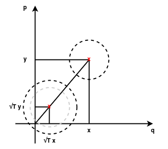
Representation of the coherent state in the phase space, after transmission

The excess noise \(\xi\) is one of the most important parameter in CV-QKD. The reason for this noise is two-fold: first, in the physical world, there is a large number of reasons for added noise when transmitting states through a fiber or a free space link. This article [LPF+18] presents some effects that participate in the excess noise. The second source is the eavesdropper: any measurement will add noise to the quantum states. Hence if we make the assumption that all the noise is coming from the eavesdropper, it is possible, using Holevo’s bound to find the maximal amount of information an eavesdropper has gained, if it had made measurements leading to the noise \(\xi\).

Note

An eavesdropper could perform non-Gaussian attacks, which would made the channel non Gaussian. However it can be proven, that if a Gaussian modulation is used, the optimal attacks for Eve are Gaussian attacks, meaning that the analysis can be restricted to this case.

Attributing all this excess noise \(xi\) to the eavesdropper, it is possible to bound the information that was gained by an eavesdropper using Holevo’s bound \(\chi_{BE}\). This allows to find the formula for the secret key rate with the Devetak-Winter formula [DW05]:

\[K = \beta I_{AB}(V_A, T, \xi, \eta, V_{el}) - \chi_{BE}(V_A, T, \xi, \eta, V_{el})\]

where \(\beta\) is the efficiency of the error correction protocol (also called reconciliation efficiency), \(V_A\) the modulation strength of Alice, which is twice the average number of photons per symbol, \(V_A = 2\cdot\langle n \rangle\), \(T\) is the transmittance of the channel, \(\xi\) is the excess noise of the channel, \(\eta\) is the efficiency of the detector and \(V_{el}\) is the electronic noise of the receiver. \(I_{AB}\) corresponds the amount of information shared between Alice and Bob and can be computed using Shannon’s theory as \(\log(1+\text{SNR})\) where SNR is the Signal to Noise Ratio. \(\chi_{BE}\) corresponds to the maximal amount of information shared between Bob and Eve [1]. This gives the secret key rate in bits per symbol, and then need to be multiplied by the symbol rate to get the secret key rate in bits per second [2].

Hence the protocol can be summarized as follow: Alice sends coherent states, with minimal noise to Bob. Bob then measures the coherent states, and estimate the added noise in the transmission. This added noise gives a bound on the information that an eavesdropper has gained during transmission, an can be removed to the quantity of information shared between Alice and Bob. Alice and Bob then use the classical channel to correct the errors (reconciliation) and remove any information that Eve has gained by compressing the key to the secret key fraction (privacy amplification).

Note

What is the different between classical coherent communication and CV-QKD? The different lies in the average number of photons per symbol \(\langle n \rangle\) or equivalently the modulation strength \(V_A\). In coherent communication, we try to maximise the signal to noise ratio, which is done by increasing \(V_A\). In CV-QKD however, doing this also gives more information to Eve, and Eve information asymptotically grows faster than the shared information between Alice and Bob. Indeed there is an optimal value for \(V_A\) given all the other parameters, that maximises the key rate. This value is usually in the order of a few photons per symbol or less.

Protocol

In the following we give the description of the CV-QKD protocol using coherent states, with Gaussian modulation:

1. Alice generates random symbol which are complex numbers with both components following a Gaussian Modulation with variance \(V_A\). Ideally, the symbols are generated using a Quantum Random Number Generator (QRNG);

2. Alice applies her Digital Signal Processing to the symbols to prepare them for Physical Transmission (see here for more details);

3. Alice generates the coherent states (for instance using an IQ modulator) and sends them to Bob through the unsecure quantum channel. Alice also measure the average number of photons per symbol \(\langle n \rangle\) using part of the generated signal;

4. Bob detects the coherent states using coherent detection;

5. Bob applies his Digital Signal Processing (see here for more details);

6. Alice sends to Bob \(\langle n \rangle\) and some of her symbols through the classical channel;

7. Bob performs the parameters estimation step to estimate \(T\) and \(\xi\) (see here for more details);

8. Bob computes the secret key rate using the estimated parameters (see here for more details). If the key rate is 0 or less, they abort. If the key rate is strictly more than zero, they continue;

9. Alice and Bob performs the error correction step (reverse reconciliation) using the classical channel (this step is not currently implemented in QOSST). At this point, Alice and Bob share an equal string of bits, but not secret;

10. Alice and Bob performs the privacy amplification step using the classical channel (this step is not currently implemented in QOSST). At this point, Alice and Bob share an equal and secret string of bits, that can be used for symmetric cryptography.

In practice, the QOSST software was planned to be use with Optical Single Sideband Gaussian Modulated Coherent States with frequency multiplexed pilots. More information can be found in the documentation of the DSP of Alice (here), the DSP of Bob (here) and the documentation of qosst-core (here).

Experimental setup

An example of an experimental setup compatible with QOSST is presented in the next figure:

Proposed scheme for CV-QKD

Alice is composed of a control computer, an DAC, an IQ modulator, a modulator controller, a beam splitter and monitoring photodiode and attenuation. The principle of the IQ modulator is 3 Mach-Zehnder interferometer. The IQ modulator requires 3 DC voltages to operate around the good functioning point. Those 3 voltages are set by the modulator controller that lock the modulator around its functioning point. The attenuation is needed ot reach the level of \(V_A\) needed for CV-QKD as explained in the previous sections.

The channel is here represented by a fiber spool.

Bob is composed on the signal input of a polarisation controller and a switch. Then the signal is mixed in a 50:50 beam splitter with a high power local oscillator. The detection is then performed by a balanced detector and recorded using an ADC. Bob also has a control computer. The polarisation controller is needed to compensate for the polarisation rotation in the fiber, as the polarisations need to be the same for the interference in the 50:50 beam splitter. The switch is needed to be able to switch to the other, non-connected input, for calibration.

Challenges in CV-QKD

In this section we quickly review some of the challenges of CV-QKD:

• DSP: the Digital Signal Processing of CV-QKD is usually one of the most important piece of software for the experiment. The goal of QOSST is to provide a base DSP for CV-QKD;

• Real Gaussian modulation does not exist, and for this reason, there is high interests, both in the theoretical and experimental part, in discret modulations such as PSK or QAM. QOSST implements those modulations and it is then possible to test those modulations with QOSST;

• Implementing the DSP, and other classical task, in real time is one of the main challenge of CV-QKD. An interface between QOSST and an FPGA was coded, meaning that this could be a possibility to increase the speed. However, QOSST was never meant to be a real time system, and the chosen programming language, python, is already a huge bottleneck;

• Increasing the achievable distance is also a greta challenge in CV-QKD especially since it performs at much lower distances than DV-QKD protocol;

• Reducing the base excess noise, by improving the DSP techniques is also a challenge;

• Finally integrating the CV-QKD transmitters and receivers is a promising and challenging technology. CV-QKD benefits from an easier integration process than its DV counterpart, and a lot of efforts is put to reach fully integrated CV-QKD systems.

---

[1]

The error correction step (or reconciliation) can be done in two settings: either Bob corrects his data to match Alice’s, which is called direct reconciliation (DR) or Alice corrects her data to match Bob’s, which is called reverse reconciliation (RR). It can be shown that protocols with Direct Reconciliation cannot exceed 3 dB (~15 km) of losses, whereas Reverse Reconciliation can theoretically go to arbitrary high levels of noise, which is why all protocols now consider Reverse Reconciliation.

[2]

Note that the actual generation key rate may be lower than this value since there are bottlenecks in the digital signal processing, error correction and privacy amplification algorithms.